Location Set Covering Problem (LSCP) - pulp method
geospatial
map
spatial optimization
Introduction
Location Set Covering Problem (LSCP) fall within a class of problems known as set covering problems. The set covering problem class is an NP-hard problem within the combinatorial optimization space. These problems typically aim at minimizing the number of sets within a space that cover all the demand within that space.
For example, the emergency services problem, where a given number of emergency service facilities must service the demand of all the residents in a given community. The emergency planning departments within this community may want to know if the demand from the community can be met with the existing infrastructure. If there are too few facilities to triage the community’s needs, then additional facilities may need to be constructed. Conversely, there may be too many facilities in the community than needed. This may present opportunities to consolidate the facilities, resulting in operational savings.
These services are often responding to emergencies that are time sensitive, such as when someone is having a heart attack or when a house is on fire. Service time and service distance are constraints that can be applied to the set covering problem, whereby you’re minimizing the number of locations that service the demand points within a specified period or service distance.
Dataset
Load dataset
For street dataset, we’ll be using a subset of the street network for Washington, DC. The street network has been pulled from Open Street Maps using the OSMNX package. Data from Open Street Map is licensed under the Open Data Commons Open Database License; more information can be found at https://www.openstreetmap.org/copyright.This dataset has been done some additional setup such as: subset it (into a spaghetti network) and reproject it ( Snapping moves the simulated point to the closest node on the network).
We generate random number and location for patients (in this project, we used 150 locations), and generate random location for three medical centers. We also calculate a distance-based cost matrix showing the distance between each patient and medical center location.
With the cost matrix calculated, you can now pass it to the code to identify the optimal medical locations to serve all of the patient demand.
streets_gpd = gpd.read_parquet(r'..\map\book\streets_gpd.parquet')
patients_snapped = gpd.read_parquet(r'..\map\book\patients_snapped.parquet')
medical_centers_snapped = gpd.read_parquet(r'..\map\book\medical_centers_snapped.parquet')

patient_locs = gpd.read_parquet(r'..\map\book\patient_locs.parquet')
medical_center_locs = gpd.read_parquet(r'..\map\book\medical_center_locs.parquet')
cost_matrix = np.loadtxt(r'..\map\book\cost_matrix.csv', delimiter=",")
Patient data
| id | geometry | comp_label | |
|---|---|---|---|
| 0 | 0 | POINT (1619991.6469726868 1923881.7353292906) | 0 |
| 1 | 1 | POINT (1619110.8295993465 1923547.2402515744) | 0 |
| 2 | 2 | POINT (1620054.6835750698 1925126.3617556223) | 0 |
| 3 | 3 | POINT (1619139.5659471645 1925343.084796712) | 0 |
| 4 | 4 | POINT (1619154.2564355868 1925714.3500127166) | 0 |
Medical centers data
| id | geometry | comp_label | |
|---|---|---|---|
| 0 | 0 | POINT (1616854.5253735012 1925670.2824466536) | 0 |
| 1 | 1 | POINT (1621140.4528528047 1923784.8131918376) | 0 |
| 2 | 2 | POINT (1616370.5274859418 1926625.6971985623) | 0 |
cost matrix
| 0 | 1 | 2 | |
|---|---|---|---|
| 0 | 4140.17 | 1573.95 | 5357.34 |
| 1 | 3892.92 | 2979.64 | 5110.08 |
| 2 | 3575.53 | 2455.77 | 4792.7 |
| 3 | 3107.27 | 3381.23 | 4324.44 |
| 4 | 3559.12 | 3661.61 | 4776.28 |
The Code
By calling maps.spatial_cluster_opt, we can identify the optimal medical locations to serve all of the patient demand.
result = maps.spatial_cluster_opt(cost_matrix, types='pulp', max_radius=5500)
This function requires the following parameters:
- main_data (
string): Data location and value - weights (
list): list of value that we want to maximize - types (
string): Type of optimization - threshold (
int): the minimum number of point each region must have - p_facilities (
int): total point (i.e. medical locations ) - max_radius (
int): maximum radius for each point
Then, byh using maps.plot_cluster_opt we can plot the results to identify which medical centers were selected and what part of the population they are serving.
maps.plot_cluster_opt(model=result,facility_points=medical_center_locs,
                    demand_points=patient_locs,map_area=streets_gpd,p_facilities=4
                    fac2cli_idx=[],types ='pulp',title="LSCP - Cost Matrix Solution"
                    center_map=[])
This function requires the following parameters:
- model (
string): result of model - facility_points (
dataframe): facility location data -
demand_points (
dataframe): demand or point location data - map_area (
dataframe): area map data - fac2cli (
dataframe): cost matrix -
p_facilities (
int): total point (i.e. medical locations ) - fac2cli_idx (
dataframe): cost matrix index - types (
string): type of plot - title (
string): title - center_map (
list):
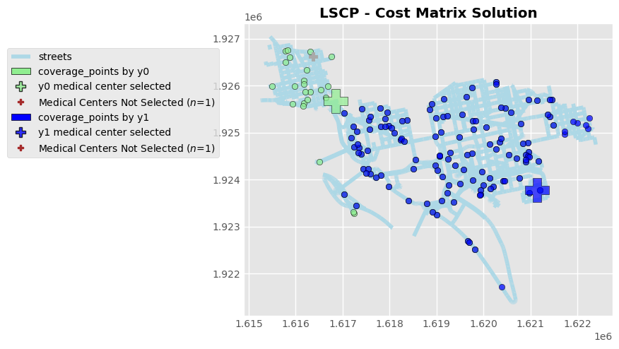
The result
We’ll notice that two medical centers can service all of the patient locations in this community, with the green medical center serving the community on the left and the blue medical center serving the community on the right. Visually, the right medical center are serving more number of people than left medical center.
The third medical center that are not selected are shaded in light gray. Based on this result, there may be an opportunity to consolidate this medical center into the left one center as it is not needed to service this community.